In this lecture we shall discuss how one can predict the future using recurrent neural networks (RNN).
RNN Introduction
RNNs are capable of handing sequential data. Sequential Data refers to any data that contain elements that are ordered into sequences.
Recurrent Neurons and Layers
A recurrent neural network looks very much like a feedforward neural network, except it also has connections pointing backward.
Feedforward NN: the activations flow only in one direction, from the input layer to the output layer
The simplest possible RNN is composed of one neuron receiving inputs, producing an output, and sending that output back to itself
Recurrent Neurons
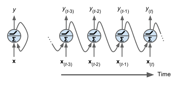
- At each time step $t$ (also called a frame), this recurrent neuron receives the inputs $x_(t)$ as well as its own output from the previous time step, $y_(t–1)$
Recurrent Layers
- A layer of recurrent neurons
- at each time step t, every neuron receives both the input vector x(t) and the output vector from the previous time step y(t–1)
Weights
- Each recurrent neuron has two sets of weights: one for the inputs x(t) and the other for the outputs of the previous time step, y(t–1).
- consider the whole recurrent layer instead of just one recurrent neuron, we can place all the weight vectors in two weight matrices, Wx and Wy
- The output of the layer $Y_{(t)}=\phi(W_x^Tx_{(t)}+W_y^T y_{(t-1)}+b)$
- NOTES
- Y(t) is a function of all the inputs since time t = 0: X(0), X(1), …, X(t)
- which means it has a form of memory.
Memory cell
- A part of a neural network that preserves some state across time steps is called a memory cell (or simply a cell)
- A single recurrent neuron, or a layer of recurrent neurons, is a very basic cell, capable of learning only short patterns (typically about 10 steps long, but this varies depending on the task)
- In general a cell’s state at time step t, denoted $h(t)$ (the “h” stands for “hidden”), is a function of some inputs at that time step and its state at the previous time step: $h(t) = f(h(t–1), x(t))$.
- Its output at time step t, denoted $y(t)$, is also a function of the previous state and the current inputs
- in basic cells, $y(t)=h(t)$
Different RNN structures
- Sequence-to-sequence network
- RNN takes a sequence of inputs and produce a sequence of outputs.
- example: predicting time series such as stock prices
sequence: the elements have order
- Sequence-to-vector network
- feed the network a sequence of inputs and ignore all outputs except for the last one
- example: feed the network a sequence of words corresponding to a movie review, and the network would output a sentiment score
- vector-to-sequence network
- could feed the network an input vector and let the network output a sequence
- example: the input could be an image (or the output of a CNN), and the output could be a caption for that image.
- Encoder-decoder two step model
- sequence-to-vector network, called an encoder, followed by a vector-to-sequence network, called a decoder
- example: translating a sentence from one language to another
Training RNNs
backpropagation through time (BPTT): unroll RNN through time and then simply use regular backpropagation
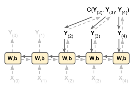
- there is a first forward pass through the unrolled network - dashed arrows
- Then the output sequence is evaluated using a cost function $C(Y(0), Y(1), …, Y(T))$
- Note that this cost function may ignore some outputs
- The gradients of that cost function are then propagated backward through the unrolled network - solid arrows.
- Finally the model parameters are updated using the gradients computed during BPTT
Implementing a Simple RNN
1
2
3
# a single layer, with a single neuron
model = keras.models.Sequential([ keras.layers.SimpleRNN(1, input_shape=[None, 1])
])
- first input dimension is None: We do not need to specify the length of the input sequences (unlike in the previous model), since a recurrent neural network can process any number of time steps
- By default, the SimpleRNN layer uses the hyperbolic tangent activation function
- By default, recurrent layers in Keras only return the final output. To make them return one output per time step, you must set
return_sequences=True
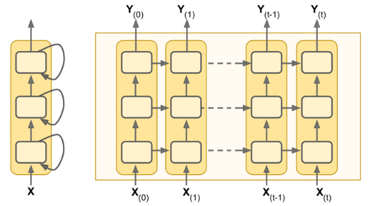
Deep RNNs
It is quite common to stack multiple layers of cells - a deep RNN
1
2
3
model = keras.models.Sequential([ keras.layers.SimpleRNN(20, return_sequences=True, input_shape=[None, 1]),
keras.layers.SimpleRNN(20, return_sequences=True), keras.layers.SimpleRNN(1)
])
Make sure to set return sequences=True for all recurrent layers
Problem with Simple RNNs
- Simple RNNs can be quite good at forecasting time series or handling other kinds of sequences, but they do not perform as well on long time series or sequences.
- To train an RNN on long sequences, we must run it over many time steps, making the unrolled RNN a very deep network. Just like any deep neural network it may suffer from the unstable gradients problem
- Moreover, when an RNN processes a long sequence, it will gradually forget the first inputs in the sequence.
- Solutions for unstable gradients problem
- good parameter initialization, faster optimizers, dropout
- nonsaturating activation functions (e.g., ReLU) lead the RNN to be even more unstable during training
- can reduce this risk by using a smaller learning rate,
- you can also simply use a saturating activation function like the hyperbolic tangent
- If you notice that training is unstable, you may want to monitor the size of the gradients (e.g., using TensorBoard) and perhaps use Gradient Clipping.
- Batch Normalization cannot be used between time steps
- layer normalization: it normalizes across the features dimension
- it can compute the required statistics on the fly, at each time step, independently for each instance
- it behaves the same way during training and testing (as opposed to BN)
- In an RNN, it is typically used right after the linear combination of the inputs and the hidden states
- solutions for short-term memory problem
- various types of cells with long-term memory have been introduced: LSTM, GRU. They have proven so successful that the basic cells are not used much anymore
Long-term memory Cells
LSTM cells
- Long Short-Term Memory
- advantages
- perform much better;
- training will converge faster,
- it will detect long-term dependencies in the data
-
structure
-
The key idea is that the network can learn what to store in the long-term state, what to throw away, and what to read from it
- The long-term state $c(t-1)$ first goes through a forget gate, dropping some memories, and then it adds some new memories via the addition operation (which adds the memories that were selected by an input gate).
- The result c(t) is sent straight out, without any further transformation.
-
-
Three gates
- use the logistic activation function, if they output 0s they close the gate, and if they output 1s they open it
-
Summary
- an LSTM cell can learn to recognize an important input (that’s the role of the input gate), store it in the long-term state, preserve it for as long as it is needed (that’s the role of the forget gate), and extract it whenever it is needed
-
Variant of LSTM
- In a regular LSTM cell, the gate controllers can look only at the input x(t) and the previous short-term state h(t–1)
- peephole connections
- the previous long-term state c(t–1) is added as an input to the controllers of the forget gate and the input gate,
- the current long-term state c(t) is added as input to the controller of the output gate.
tf.keras.experimental.PeepholeLSTMCellin Keras
GRU cells
- Gated Recurrent Unit cell
- a simplified version of the LSTM cell
- A single gate controller z(t) controls both the forget gate and the input gate
- There is no output gate; the full state vector is output at every time step.
- new gate controller r(t) that controls which part of the previous state will be shown to the main layer g(t).
Problems with LSTM and GRU
They still have a fairly limited short-term memory, and they have a hard time learning long-term patterns in sequences of 100 time steps or more, such as audio samples, long time series, or long sentences.
- One way to solve this is to shorten the input sequences, for example using 1D convolutional layers.
- use “valid” padding or a stride greater than 1, then the output sequence will be shorter than the input sequence
WaveNet
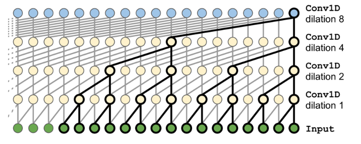
- use only 1D convolutional layers and drop the recurrent layers entirely
- 1D convolutional layers are stacked doubling the dilation rate (how spread apart each neuron’s inputs are) at every layer
- the lower layers learn short-term patterns, while the higher layers learn long-term patterns
- WaveNet architecture was successfully applied to various audio tasks, including text-to-speech tasks, producing incredibly realistic voices across several languages, generating music, one audio sample at a time.