Convolutional neural networks (CNNs) are not restricted to visual perception: they are also successful at many other tasks, such as voice recognition and natural language processing. This blog focus visual applications of CNN.

CNN Architectures

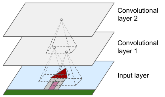
Convolutional layers

The most important building block of a CNN
Neurons in the first convolutional layer are not connected to every single pixel in the input image (like they were in the dense layers before), but only to pixels in their receptive fields
In turn, each neuron in the second convolutional layer is connected only to neurons located within a small rectangle in the first layer
In a CNN each layer is represented in 2D, which makes it easier to match neurons with their corresponding inputs

Benefit:

allows the network to concentrate on small low-level features in the first hidden layer
then assemble them into larger higher-level features in the next hidden layer

Zero Padding

Usually the height and width of the next layer will be smaller than the previous layer
In order for a layer to have the same height and width as the previous layer, it is common to add zeros around the inputs

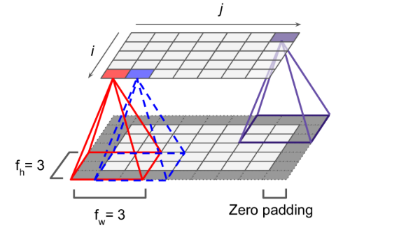
Stride

The shift from one receptive field to the next is called the stride.
We can use stride to space out the receptive fields so that we can connect a large input layer to a much smaller layer.
the stride can be different in different directions
For example
- stride=2, 5*7 input layer can be connected to a 3*4 layer with 3*3 receptive fields (plus zero padding)

Filters

A neuron’s weights can be represented as a small image the size of the receptive field. The weights are called filters or convolution kernels.
a layer full of neurons using the same filter outputs a feature map
you do not have to define the filters manually
- during training the convolutional layer will automatically learn the most useful filters for its task
- the layers above will learn to combine them into more complex patterns.

Stacking Multiple feature maps

A convolutional layer

has multiple filters
outputs one feature map per filter

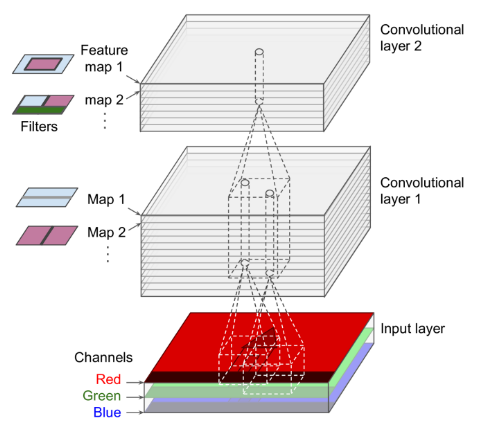
All neurons within a given feature map share the same parameters (weights and bias).
- dramatically reduces the number of parameters in the model.
A convolutional layer simultaneously applies multiple trainable filters to its inputs
Input images are also composed of multiple sublayers: one per color channel. (RGB three channel)

conv = keras.layers.Conv2D(filters=32, kernel_size=3, strides=1, padding="same", activation="relu")

# padding = "valid" means no padding

DNN vs CNN

Once the CNN has learned to recognize a pattern in one location, it can recognize it in any other location
once a regular DNN has learned to recognize a pattern in one location, it can recognize it only in that particular location

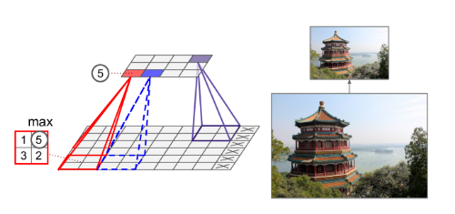
Pooling layers

Goal
- subsample the image to reduce the computational load, the memory usage, and the number of parameters
characteristics
- a pooling neuron has no weights
- all it does is aggregate the inputs using an aggregation function such as the max or mean
Types of pooling layer
- Max pooling layer
  - Only the max input value in each receptive field makes it to the next layer
- average pooling layer
- global average pooling layer
  - computes the mean of each entire feature map
  - It can sometimes be useful as an output layer
Notes
- max and average pooling layer can be performed along the depth dimension and the spatial dimensions
- When apply along the depth dimension, CNN can learn to be invariant to various features
- The stride in pooling layers is the same as the kernel size so that there is no overlap in receptive fields.

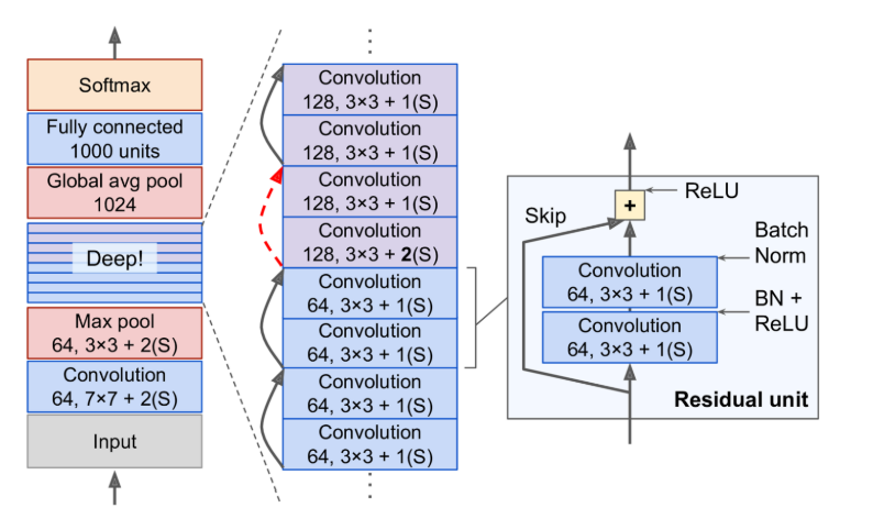
CNN architectures

the number of filters grows as we climb up the CNN toward the output layer (it is initially 64, then 128, then 256)
It is a common practice to double the number of filters after each pooling layer: since a pooling layer divides each spatial dimension by a factor of 2, we can afford to double the number of feature maps in the next layer without fear of exploding the number of parameters, memory usage, or computational load
On the top there is a fully connected network, composed of two hidden dense layers and a dense output layer
- we must flatten its inputs, since a dense network expects a 1D array of features for each instance

Different CNN architectures

LeNet-5

used for handwritten digit recognition by the post office.
average pooling layers
- each neuron computes the mean of its inputs, then multiplies the result by a learnable coefficient (one per map) and adds a learnable bias term (again, one per map),
- Most neurons in C3 maps are connected to neurons in only three or four S2 maps (instead of all six S2 maps)
output layer
- each neuron outputs the square of the Euclidian distance between its input vector and its weight vector.
- Each output measures how much the image belongs to a particular digit class
The cross-entropy cost function is now preferred
- it penalizes bad predictions much more,
- producing larger gradients and converging faster

AlexNet

similar to LeNet-5 while larger and deeper
regularization techniques
- dropout with a 50% dropout rate applied to the outputs of layers F9 and F10
- data augmentation by randomly shifting the training images by various offsets, flipping them horizontally, and changing the lighting conditions
local response normalization: a competitive normalization step immediately after the ReLU step of layers C1 and C3
- the most strongly activated neurons inhibit other neurons located at the same position in neighboring feature maps
- this encourages different feature maps to specialize, pushing them apart and forcing them to explore a wider range of features, ultimately improving generalization.

GoogLeNet

This great performance came in large part from the fact that the network was much deeper than previous CNNs
This was made possible by subnetworks called inception modules
- allow GoogLeNet to use parameters much more efficiently than previous architectures
- the second set of convolutional layers uses different kernel sizes (1 × 1, 3 × 3, and 5 × 5), allowing them to capture patterns at different scales.
Why 1 × 1 kernels are used?
- Although they cannot capture spatial patterns, they can capture patterns along the depth dimension.

VGGNet

It had a very simple and classical architecture, with 2 or 3 convolutional layers and a pooling layer, then again 2 or 3 convolutional layers and a pooling layer, and so on
It used only 3 × 3 filters, but many filters

ResNet

skip connections (shortcut connections)
- the signal feeding into a layer is also added to the output of a layer located a bit higher up the stack
Benefits
- When you initialize a regular neural network, its weights are close to zero, so the network just outputs values close to zero.
- If you add a skip connection, the resulting network just outputs a copy of its inputs; in other words, it initially models the identity function
- this will speed up training considerably
The deep residual network can be seen as a stack of residual units (RUs)

Xception (Extreme Inception)

it significantly outperformed Inception-v3 on a huge vision task
merges the ideas of GoogLeNet and ResNet
- replaces the inception modules with a special type of layer called a depthwise separable convolution layer
a separable convolutional layer makes the strong assumption that spatial patterns and cross-channel patterns can be modeled separately
- a regular convolutional layer uses filters that try to simultaneously capture spatial patterns (e.g., an oval) and cross-channel patterns

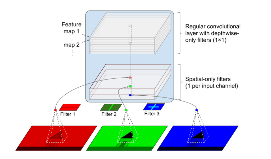
it is composed of two parts
- the first part applies a single spatial filter for each input feature map
- the second part looks exclusively for cross-channel patterns
Since separable convolutional layers only have one spatial filter per input channel, you should avoid using them after layers that have too few channels, such as the input layer.

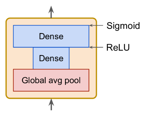
SENet

This architecture extends existing architectures such as inception networks and ResNets, and boosts their performance
The boost comes from the fact that a SENet adds a small neural network, called an SE block, to every unit in the original architecture (i.e., every inception module or every residual unit)
SE block
- An SE block analyzes the output of the unit it is attached to, focusing exclusively on the depth dimension
- it learns which features are usually most active together
- uses this information to recalibrate the feature maps
- An SE block is composed of just three layers: a global average pooling layer, a hidden dense layer using the ReLU activation function, and a dense output layer using the sigmoid activation function

Object detection

Intro

The task of classifying and localizing multiple objects in an image is called object detection.

Metrics

The MSE often works fairly well as a cost function to train the model, but it is not a great metric to evaluate how well the model can predict bounding boxes.
Intersection over Union (IoU)
- the area of overlap between the predicted bounding box and the target bounding box, divided by the area of their union.
- tf.keras.metrics.MeanIoU
Mean Average Precision (mAP)
- the precision/recall curve may contain a few sections where precision actually goes up when recall increases, especially at low recall values
- This is one of the motivations for the mAP metric
- compute the maximum precision you can get with at least 0% recall, then 10% recall, 20%, and so on up to 100%, and then calculate the mean of these maximum precisions. This is called the Average Precision (AP) metric.
- what if the system detected the correct class, but at the wrong location?
  - One approach is to define an IOU threshold: for example, we may consider that a prediction is correct only if the IOU is greater than, say, 0.5, and the predicted class is correct: mAP

Approaches

take a CNN that was trained to classify and locate a single object, then slide it across the image
non-max suppression
- steps
  - First, you need to add an extra objectness output to your CNN, to estimate the probability that a flower is indeed present in the image
  - sigmoid activation function
  - then drop all the bounding boxes that don’t actually contain a flower.
  - Find the bounding box with the highest objectness score
  - get rid of all the other bounding boxes that overlap a lot with it
  - Repeat step two until there are no more bounding boxes to get rid of.
- drawbacks
  - slow
fully convolutional network (FCN)
- replace the dense layers at the top of a CNN by convolutional layers.
- it can be trained and executed on images of any size
- the FCN approach is much more efficient than sliding, since the network only looks at the image once
You Only Look Once (YOLO)
- similar to FCN with the following differences
  - YOLOv3 algorithm (there are two older versions) outputs five bounding boxes for each grid cell
  - It also outputs 20 class probabilities per grid cell
- YOLOv3 predicts an offset relative to the coordinates of the grid cell
- Before training the neural net, YOLOv3 finds five representative bounding box dimensions, called anchor boxes (or bounding box priors) by K-Means

Machine Learning: CNN

CNN introduction and Common Architectures