Problems with training DNN
Problems
Training deeper networks consisting of 10s or 100s layers runs into the following problems:
- Vanishing gradient problem
- gradients get smaller and smaller from layer to layer
- Exploding gradient problem
- gradients get larger and larger
Both these problems will make training extremely slow.
Reasons
- Sigmoid-like activation functions
- One reason for vanishing gradients is using a sigmoid-like activation function in the hidden layers
- When inputs become large (negative or positive), the function saturates at 0 or 1, with a derivative extremely close to 0
- simple random initialization
- simple random initialization from a normal distribution contributes to the problem of vanishing/exploding gradients
Other weight initialization and activation functions
-
weight initialization
initialization explain note Glorot (Xavier) The weights of a layer are initialized either from a normal distribution with mean 0 and variance $\sigma^2=1/fan_{avg}$ or from a uniform distribution 1between −r and +r where $r=\sqrt{3/fan_{avg}}$ $fan_{in}$ is the number of inputs of the layer; $fan_{out}$ is the number of outputs of the layer LeCun the weights for a layer are taken from a normal distribution with mean 0 and variance $\sigma^2=1/fan_{in}$ Must be used when using SELU as activation function He the weights for a layer are taken from a normal distribution with mean 0 and variance $\sigma^2=2/fan_{in}$ or from a uniform distribution -
Non-saturating activation functions
name explain problem ReLU helps to avoid saturation; dying ReLUs: during training, some neurons effectively “die”: they stop outputting anything other than 0. LeakyReLU $LeakyReLU_α(z) = max(αz, z)$ Randomized leaky ReLU (RReLU) $α$ is picked randomly in a given range during training; is fixed to an average value during testing Parametric leaky ReLU (PReLU) α is a parameter to be learned during training Exponential linear unit (ELU): 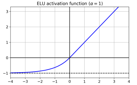
Scaled ELU (SELU) if all hidden layers (must be dense layer) use the SELU activation function, then the network will self-normalize and solve the vanishing/exploding gradients problem (1)The input features must be standardized (mean 0 and standard deviation 1); (2) LeCun normal initialization; (3) sequential architecture -
Preferences
SELU > ELU > leaky ReLU (and its variants) > ReLU > tanh> logistic
Batch Normalization
Using different initialization or activation functions can significantly reduce the danger of the vanishing/exploding gradients problems at the beginning of training, it doesn’t guarantee that they won’t come back during training.
- BN is added either before or after applying activation function
- the operation lets the model learn the optimal scale and mean of each of the layer’s inputs.
- steps
- BN zero-centers and normalizes each input
- then scales and shifts the result using two new parameter vectors per layer
-
if you add a BN layer as the very first layer of your neural network, you do not need to standardize your training set
- how to make predications
- During training, BN collects statistics to compute mean and std on the whole dataset.
- four parameter vectors are learned in each batch-normalized layer: $\gamma$, $\beta$, $\mu$ and $\sigma$
- $µ$ and $σ$ are estimated during training, but they are used only after training to replace the batch input means and standard deviations
- hyperparameters
- momentum: compute moving average of the vector v (mean and std)
- axis: which axis should be normalized. Default: -1
- pros
- makes training less sensitive to weight initialization
- typically improves the convergence
- acts as a regularization
- downside
- requires more computations
- but it might be compensated by faster convergence
Gradient Clipping
-
Another popular technique to mitigate the exploding gradients problem is to clip the gradients during backpropagation so that they never exceed some threshold
-
used in RNN (batch normalization is tricky to use in RNNs)
-
implementation in keras
-
1
2
3
optimizer = keras.optimizers.SGD(clipvalue=1.0) model.compile(loss="mse", optimizer=optimizer)

# or use clip norm
-
clipvaluemight significantly change the orientation of the gradient clipnormcan keep the orientation and clip the length
-
Transfer Learning
- Def
- find an existing neural network that accomplishes a similar task to the one you are trying to tackle
- then reuse the lower layers of this network.
- Benefits
- speed up training considerably
- require significantly less training data
- process
- replace the output layer
- the upper hidden layers of the original model are less likely to be as useful as the lower layers
- the high-level features that are most useful for the new task may differ significantly from the ones that were most useful for the original task.
- Try freezing all the reused layers first
- then train your model and see how it performs.
- Then try unfreezing one or two of the top hidden layers to let backpropagation tweak them and see if performance improves.
- Notes
- It is also useful to reduce the learning rate when you unfreeze reused layers
- this will avoid wrecking their fine-tuned weights
Not enough labeled data
Option 1: unsupervised pretraining
- If you can gather plenty of unlabeled training data, you can try to use it to train an unsupervised model
- such as an autoencoder or a generative adversarial network
- Then you can reuse the lower layers of the autoencoder or the lower layers of the GAN’s discriminator
- add the output layer for your task on top,
- fine-tune the final network using supervised learning
Option 2: pretraining on an auxiliary task
- train a first neural network on an auxiliary task for which you can easily obtain or generate labeled training data
- then reuse the lower layers of that network for your actual task
- example
- task: recognize faces
- auxiliary task: detect whether or not two different pictures feature the same person
- Such a network would learn good feature detectors for faces, so reusing its lower layers would allow you to train a good face classifier that uses little training data.
Self-supervised learning
- when you automatically generate the labels from the data itself, then you train a model on the resulting “labeled” dataset using supervised learning techniques.
- This approach requires no human labeling
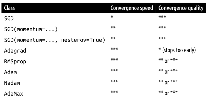
Fast Optimizers
-
Momentum Optimization
- The next step is determined by both the local gradient and also the previous momentum
-
Nesterov momentum optimization
- measures the gradient of the cost function not at the local position $θ$ but slightly ahead in the direction of momentum $θ + βm$
-
AdaGrad algorithm
- could correct the direction earlier to point a bit more toward the global optimum
-
Adaptive learning rate: AdaGrad algorithm decays the learning rate. And it does so faster for steep dimensions than for dimensions with gentler slopes
- Benefit
- requires much less tuning of the learning rate hyperparameter
- drawbacks
- stops too early when training neural networks
-
RMSProp
- accumulating only the gradients from the most recent iterations
- It does so by using exponential decay in the first step
- This fixes the problem of AdaGrad where it might never converges to the global optimum
- RMSProp almost always outperforms AdaGrad
-
Adam (adaptive moment estimation)
- combines the ideas of momentum optimization and RMSProp
- Adam scales down the parameter updates by the l2 norm of the time-decayed gradients
-
AdaMax
- use another way to scales down the parameter updates
- more stable than Adam
- really depends on the dataset, and in general Adam performs better
-
Nadam optimization
- Adam optimization plus the Nesterov trick
- often converge slightly faster than Adam.
-
summary
Learning Rate scheduling
What is learning rate scheduling?
Finding a good learning rate is very important.
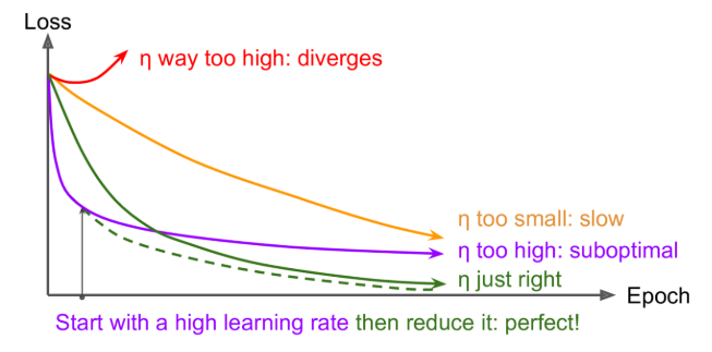
Learning schedules: start with a large learning rate and then reduce it once training stops making fast progress, you can reach a good solution faster than with the optimal constant learning rate
Types of learning rate scheduling
- power scheduling
- This schedule first drops quickly, then more and more slowly.
- exponential scheduling
- $η$ will gradually drop by a factor of 10 every $s$ steps
- Piecewise constant scheduling
- Use a constant $η$ for a number of epoch, then - a smaller one for a number of epochs, etc
- performance scheduling
- Measure the validation error every N steps
- then reduce the learning rate by a factor of $λ$ when the error stops dropping
- 1cycle scheduling
Summary
exponential decay, performance scheduling, and 1cycle can considerably speed up convergence
Avoid Overfitting
l1,l2 regularization
- We can use l1 and l2 regularization for neural networks
- These regularizations are applied to the weights of each layer
Dropout
- At every training step, every neuron (including the input neurons, but always excluding the output neurons) has a probability p of being temporarily “dropped out”, meaning it will be entirely ignored during this training step, but it may be active during the next step
- A unique neural network is generated at each training step.
- The resulting neural network can be seen as an averaging ensemble of all these smaller neural networks.
- The hyperparameter p is called the dropout rate, and it is typically set between 10% and 50%:
- closer to 20-30% in recurrent neural nets and closer to 40–50% in convolutional neural networks
- After training, neurons don’t get dropped anymore
- Alpha dropout
- If you want to regularize a self-normalizing network based on the SELU activation function, you should use alpha dropout: this is a variant of dropout that preserves the mean and standard deviation of its inputs
Monte Carlo Dropout
- MC Dropout can boost the performance of any trained dropout model without having to retrain it or even modify it at all, provides a much better measure of the model’s uncertainty, and is also amazingly simple to implement.
- acts the same during training and prediction
- allow random dropout during prediction
- But instead of using one result of NN, we are using the ensemble result for prediction.