Artificial Neural Networks (ANN) is a Machine Learning model inspired by the networks of biological neurons found in our brains

The Perceptron

one of the simplest ANN architectures
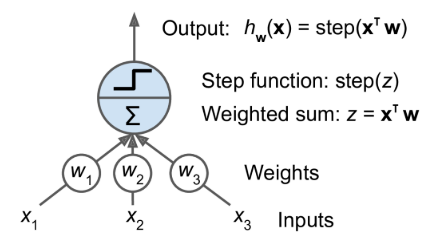
Threshold logic unit (TLU): also called a linear threshold unit
- TLU computes a weighted sum of its inputs, then applies a step function
- A single TLU can be used for simple linear binary classification

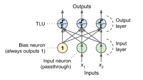
Perceptron
- composed of a single layer of TLUs
- each TLU connects to all the inputs
- All the input neurons form the input layer.
- an extra bias feature is generally added (x0 = 1): it is typically represented using a special type of neuron called a bias neuron, which outputs 1 all the time
structure
formula for outputs
- \[h_{W,b}(X)=\phi(XW+b)\]
- $X$: input features, one row per instance, one col per feature
- $W$: connection weights except for the one from the bias neuron (yellow circle) , one row per neuron, one col per unit in the layer
- $b$: all the connection weights between the bias neuron and the neurons in the output layer
- $\phi$: the activation function: when the artificial neurons are TLUs, it is a step function
learning rule
- The Perceptron is fed one training instance at a time
- for each instance it makes its predictions and adjusts the weights
- Linear decision boundary, only solve linearly separable problem
Notes
- Perceptrons make predictions based on a hard threshold,

Multilayer Perceptron (MLP)

Intro
- stacking multiple Perceptrons, each layer has a bias neuron
- allows to handle complicated decision boundaries
- Also called feedforward neural network or fully connected neural network
Backpropagation
- the backpropagation algorithm is able to compute the gradient of the network’s error with regard to every single model parameter
- It handles one mini-batch at a time, and it goes through the full training set multiple times. Each pass is called an epoch
- steps when training NN
  - Each mini-batch is passed to the network’s input layer, we get the output of the last layer, the output layer (forward pass)
  - Next, the algorithm measures the network’s output error
  - Then the algorithm measures how much each connection contributed to the error and uses the chain rule working backward until reaching the input layer
  - finally the algorithm performs a Gradient Descent step to tweak all the connection weights in the network, using the error gradients it just computed.
- Notes
  - It is important to initialize all the hidden layers’ connection weights randomly, or else training will fail
Activation functions
- sigmoid function
- hyperbolic tangent function $tanh(z)=2\sigma(2z)-1$
  - S-shaped, continuous and differentiable like sigmoid function
  - ranges from -1 to 1
  - each layer’s output more or less centered around 0 at the beginning of training, which often helps speed up convergence
- Rectified Linear Unit Function $ReLU(z)=max(0,z)$
  - continuous, not differentiable at z=0
  - In practice, it works very well and has the advantage of being fast to compute, so it has become the default
  - it does not have a maximum output value so that it helps reduce some issues during Gradient Descent
Regression MLP
- output layer
  - single value: a single output neuron
  - multivariate regression: one output neuron per output dimension
- activation function
  - don’t use any activation function for the output neurons so the NN are free to output any range of values
  - use ReLU in the output layer when output need to be positive
    - or softplus (a smooth variant of ReLU)
  - 0-1 range output: sigmoid function
  - -1 - 1range output: hyperbolic tangent
- Loss function
  - MSE
  - many outliers: MAE
  - combination of both: Huber loss
Classification MLP
- binary
  - a single output neuron
  - logistic function
- multiclass
  - 1 neuron per class
  - softmax function
- multilabel binary
  - 1 per label
  - logistic function
- Loss function
  - cross-entropy loss

Implementing MLPs with Keras

Sequential API

import tensorflow as tf
from tensorflow import keras

# method 1
model = keras.models.Sequential()
model.add(keras.layers.Flatten(input_shape=[28, 28]))
model.add(keras.layers.Dense(300, activation="relu"))
model.add(keras.layers.Dense(100, activation="relu"))
model.add(keras.layers.Dense(10, activation="softmax"))

# method 2
model = keras.models.Sequential([
    keras.layers.Flatten(input_shape=[28, 28]),
    keras.layers.Dense(300, activation="relu"),
    keras.layers.Dense(100, activation="relu"),
    keras.layers.Dense(10, activation="softmax")
])

# plot model
keras.utils.plot_model(model, to_file="my_fashion_mnist_model.png", show_shapes=True)

# compile model
model.compile(loss="sparse_categorical_crossentropy",optimizer="sgd",metrics=["accuracy"])

# fit model
history = model.fit(X_train, y_train, epochs=30,
                    validation_data=(X_valid, y_valid))

# plot learning curves
import pandas as pd

pd.DataFrame(history.history).plot(figsize=(8, 5))
plt.grid(True)
plt.gca().set_ylim(0, 1)
save_fig("keras_learning_curves_plot")
plt.show()

Functional API

Could be used to build complex models
- Wide and Deep NN: this architecture makes it possible for the neural network to learn both deep patterns (using the deep path) and simple rules (through the short path)
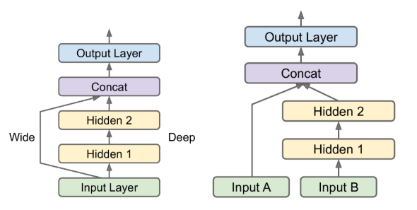
- add some auxiliary outputs in a neural network architecture to ensure that the underlying part of the network learns something useful on its own, without relying on the rest of the network.
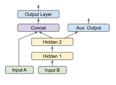
code

# wide&deep nn
input_ = keras.layers.Input(shape=X_train.shape[1:])
hidden1 = keras.layers.Dense(30, activation="relu")(input_)
hidden2 = keras.layers.Dense(30, activation="relu")(hidden1)
concat = keras.layers.concatenate([input_, hidden2])  # connect input and output directly
output = keras.layers.Dense(1)(concat)
model = keras.models.Model(inputs=[input_], outputs=[output])

# multiple input
input_A = keras.layers.Input(shape=[5], name="wide_input")
input_B = keras.layers.Input(shape=[6], name="deep_input")
hidden1 = keras.layers.Dense(30, activation="relu")(input_B)
hidden2 = keras.layers.Dense(30, activation="relu")(hidden1)
concat = keras.layers.concatenate([input_A, hidden2])
output = keras.layers.Dense(1, name="output")(concat)
model = keras.models.Model(inputs=[input_A, input_B], outputs=[output])

# wide&deep nn and auxiliary output
input_A = keras.layers.Input(shape=[5], name="wide_input")
input_B = keras.layers.Input(shape=[6], name="deep_input")
hidden1 = keras.layers.Dense(30, activation="relu")(input_B)
hidden2 = keras.layers.Dense(30, activation="relu")(hidden1)
concat = keras.layers.concatenate([input_A, hidden2])
output = keras.layers.Dense(1, name="main_output")(concat)
aux_output = keras.layers.Dense(1, name="aux_output")(hidden2)
model = keras.models.Model(inputs=[input_A, input_B],
                           outputs=[output, aux_output])

Subclassing API

Both the Sequential API and the Functional API are declarative
- start by declaring which layers you want to use and how they should be connected
- then can you start feeding the model some data for training or inference
- pros
  - the model can easily be saved, cloned, and shared
  - its structure can be displayed and analyzed
  - the framework can infer shapes and check types
  - It’s also fairly easy to debug
dynamic models
- Some models involve loops, varying shapes, conditional branching, and other dynamic behaviors
- notes
  - your model’s architecture is hidden within the call() method, so Keras cannot easily inspect it
  - cannot save or clone it
  - don’t know how layers are connected with each other
  - it is easier to make mistakes

class WideAndDeepModel(keras.models.Model):
    def __init__(self, units=30, activation="relu", **kwargs):
        super().__init__(**kwargs)
        self.hidden1 = keras.layers.Dense(units, activation=activation)
        self.hidden2 = keras.layers.Dense(units, activation=activation)
        self.main_output = keras.layers.Dense(1)
        self.aux_output = keras.layers.Dense(1)
        
    def call(self, inputs):
        input_A, input_B = inputs
        hidden1 = self.hidden1(input_B)
        hidden2 = self.hidden2(hidden1)
        concat = keras.layers.concatenate([input_A, hidden2])
        main_output = self.main_output(concat)
        aux_output = self.aux_output(hidden2)
        return main_output, aux_output

model = WideAndDeepModel(30, activation="relu")

Saving and Restoring models

# static models
model.save("my_keras_model.h5")
model = keras.models.load_model("my_keras_model.h5")

# dynamic models
model.save_weights("my_keras_weights.ckpt")
model.load_weights("my_keras_weights.ckpt")

Callbacks

Intro

The fit() method accepts a callbacks argument that lets you specify a list of objects that Keras will call
- at the start and end of training,
- at the start and end of each epoch,
- and before and after processing each batch

ModelCheckpoint

the ModelCheckpoint callback saves checkpoints of your model at regular intervals during training, by default at the end of each epoch
you can set save_best_only=True when creating the ModelCheckpoint, it will only save your model when its performance on the validation set is the best so far

checkpoint_cb = keras.callbacks.ModelCheckpoint("my_keras_model.h5") 
history = model.fit(X_train, y_train, epochs=10, callbacks=[checkpoint_cb])

EarlyStopping

It will interrupt training when it measures no progress on the validation set for a number of epochs (defined by the patience argument), and it will optionally roll back to the best model.

checkpoint_cb =
keras.callbacks.ModelCheckpoint("my_keras_model.h5", save_best_only=True)
    
early_stopping_cb = keras.callbacks.EarlyStopping(patience=10, restore_best_weights=True)
    
history = model.fit(X_train, y_train, epochs=100, validation_data=(X_valid, y_valid), callbacks=[checkpoint_cb, early_stopping_cb])

Customized callbacks

class PrintValTrainRatioCallback(keras.callbacks.Callback): 
    def on_epoch_end(self, epoch, logs): 
        ratio = logs["val_loss"] / logs["loss"]) 
        print(f"\nval/train: {ratio}")

also can implement
- on_train_begin()
- on_epoch_begin()
- on_batch_begin()
- on_test_begin() (called by evaluate())
- on_test_batch_begin()
- on_predict_begin() (called by predict())

TensorBoard

root_logdir = os.path.join(os.curdir, "my_logs")

def get_run_logdir():
    import time
    run_id = time.strftime("run_%Y_%m_%d-%H_%M_%S")
    return os.path.join(root_logdir, run_id)

run_logdir = get_run_logdir()
run_logdir

## tensorboard callbacks
tensorboard_cb = keras.callbacks.TensorBoard(run_logdir)
history = model.fit(X_train, y_train, epochs=30,
                    validation_data=(X_valid, y_valid),
                    callbacks=[checkpoint_cb, tensorboard_cb])

# in jupyter notebook
%load_ext tensorboard
%tensorboard --logdir=./my_logs --port=6006 --host=0.0.0.0

Hyperparameter tuning

number of hidden layers
- start with just one or two hidden layers
- For more complex problems, you can ramp up the number of hidden layers until you start overfitting the training set.
number of neurons per hidden layer
- The number of neurons in the input and output layers is determined by the type of input and output your task requires
- typically puts the same number of neurons in each hidden layer
- it’s often simpler and more efficient to pick a model with more layers and neurons than you actually need, then use early stopping and other regularization techniques to prevent it from overfitting.
learning_rate
- the optimal learning rate is about half of the maximum learning rate
  - the learning rate above which the training algorithm diverges
Optimizer
batch_size
- can have a significant impact on your model’s performance and training time
- large batch size:
  - hardware accelerators like GPUs can process them efficiently, so the training algorithm will see more instances per second
  - sizes often lead to training instabilities
  - the resulting model may not generalize as well as a model trained with a small batch size.
activation function
- in general, the ReLU activation function will be a good default for all hidden layers
number of iterations
- in most cases does not actually need to be tweaked: just use early stopping instead.

from scipy.stats import reciprocal
from sklearn.model_selection import RandomizedSearchCV
def build_model(n_hidden=1, n_neurons=30, learning_rate=3e-3, input_shape=[8]):
    model = keras.models.Sequential()
    model.add(keras.layers.InputLayer(input_shape=input_shape))
    for layer in range(n_hidden):
        model.add(keras.layers.Dense(n_neurons, activation="relu"))
    model.add(keras.layers.Dense(1))
    optimizer = keras.optimizers.SGD(lr=learning_rate)
    model.compile(loss="mse", optimizer=optimizer)
    return model

# use sklearn api
keras_reg = keras.wrappers.scikit_learn.KerasRegressor(build_model)


param_distribs = {
    "n_hidden": [0, 1, 2, 3],
    "n_neurons": np.arange(1, 100)               .tolist(),
    "learning_rate": reciprocal(3e-4, 3e-2)      .rvs(1000).tolist(),
}

rnd_search_cv = RandomizedSearchCV(keras_reg, param_distribs, n_iter=10, cv=3, verbose=2)
rnd_search_cv.fit(X_train, y_train, epochs=100,
                  validation_data=(X_valid, y_valid),
                  callbacks=[keras.callbacks.EarlyStopping(patience=10)])

Machine Learning: Artificial Neural Networks

Artificial Neural Network with Keras

The Perceptron

Multilayer Perceptron (MLP)

Implementing MLPs with Keras

Sequential API

Functional API

Subclassing API

Saving and Restoring models

Callbacks

TensorBoard

Hyperparameter tuning

CATALOG

FEATURED TAGS

FRIENDS