Unfinished

Clustering

K-Means

Algorithm
- place k centroids randomly
- label other instances by assigning them to the cluster of the closest centroid
- update centroids by computing the mean of the instances’ locations for each cluster
- repeat step 2 and 3 until the centroids stop moving

How to select initial centroids

run another clustering algorithm and know the centroids locations

good_init = np.array([[-3, 3], [-3, 2], [-3, 1], [-1, 2], [0, 2]])
kmeans = KMeans(n_clusters=5, init=good_init, n_init=1)

run the algorithm multiple times with different random initializations and keep the best solution
- by default n_init=10, which means algorithm runs 10 times and keep the best solution
- use model’s inertia to select
inertia: the mean squared distance between each instance and its closest centroid

Notes
- The algorithm is guaranteed to converge in a finite number of steps (usually quite small)
  - it may not converge to the right solution - it may converge to a local optimum: whether it does or not depends on the centroid initialization.
- K-Means algorithm does not behave very well when the blobs have very different diameters
hard and soft clustering
- hard clustering: assign each instance to a cluster
- soft clustering: give each instance a score per cluster
  - score can be the distance or similarity score (such as Gaussian Radia Basis Function)
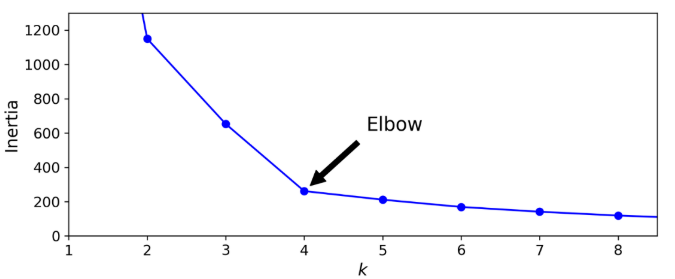
Find the optimal number of clusters
- use elbow point in inertia plot
- use sihouette score
  - vary between -1 and +1
  - $\frac{b-a}{max(a,b)}$
    - a is the mean distance to the other instances in the same cluster
    - b is the mean distance to the instances of the next closest cluster
  - +1 means the instance is well inside its own cluster and far from other clusters
  - 0 means the instance is close to a cluster boundary
  - -1 means the instance may have been assigned to the wrong cluster
  - 1 2 from sklearn.metrics import silhouette_score score = silhouette_score(X, kmeans.labels_)
  - The larger silhouette score, the better the cluster is
Limitations
- need to avoid suboptimal solutions
- need to specify k
- K-Means does not behave very well when the clusters have
  - varying sizes
  - different densities
  - nonspherical shapes.
- need to scale the input features first

Implementation

from sklearn.cluster import KMeans 
k = 5 
kmeans = KMeans(n_clusters=k) 
y_pred = kmeans.fit_predict(X)
  
kmeans.inertia_
kmeans.score(X)  # return negative inertia

K-Means++

different initialization step
- Select the first centroid uniformly randomly 2
- Select the next centroid from the data points such that the probability of choosing a point as centroid is directly proportional to its distance from the nearest, previously chosen centroid. (i.e. the point having maximum distance from the nearest centroid is most likely to be selected next as a centroid)
- Keep repeating until k centroids are chosen
Notes
- tends to select centroids that are distant from one another
- makes the K-Means algorithm much less likely to converge to a suboptimal solution

K-Means: MiniBatchKMeans

Instead of using the full dataset at each iteration, the algorithm is capable of using mini-batches, moving the centroids just slightly at each iteration
This speeds up the algorithm typically by a factor of three or four and makes it possible to cluster huge datasets that do not fit in memory.
Could combine MiniBatchKMeans with memmap if data doesn’t fit in memory
if still too large to use memmap, could use partial_fit()

Implementation

from sklearn.cluster import MiniBatchKMeans
minibatch_kmeans = MiniBatchKMeans(n_clusters=5, random_state=42)
minibatch_kmeans.fit(X)

# use memmap

## write to a memmap
filename = "my_mnist.data"
X_mm = np.memmap(filename, dtype='float32', mode='write', shape=X_train.shape)
X_mm[:] = X_train

minibatch_kmeans = MiniBatchKMeans(n_clusters=10, batch_size=10, random_state=42)
minibatch_kmeans.fit(X_mm)


# if too large to use memmap, then load one batch each time
def load_next_batch(batch_size):
    # in real life, you would load the data from disk
    return X[np.random.choice(len(X), batch_size, replace=False)]


k = 5
n_init = 10
n_iterations = 100
batch_size = 100
init_size = 500  # more data for K-Means++ initialization
evaluate_on_last_n_iters = 10

best_kmeans = None

for init in range(n_init):
# implement multiple initializations and keep the model with the lowest inertia
    minibatch_kmeans = MiniBatchKMeans(n_clusters=k, init_size=init_size)
    X_init = load_next_batch(init_size)
    minibatch_kmeans.partial_fit(X_init)

    minibatch_kmeans.sum_inertia_ = 0
    for iteration in range(n_iterations):
        X_batch = load_next_batch(batch_size)
        minibatch_kmeans.partial_fit(X_batch)
        if iteration >= n_iterations - evaluate_on_last_n_iters:
            minibatch_kmeans.sum_inertia_ += minibatch_kmeans.inertia_

    if (best_kmeans is None or
        minibatch_kmeans.sum_inertia_ < best_kmeans.sum_inertia_):
        best_kmeans = minibatch_kmeans

DBSCAN

Idea
- a clustering algorithm that illustrates a very different approach based on local density estimation
- This algorithm works well if
  - all the clusters are dense enough
  - they are well separated by low-density regions
algorithm
- For each instance, the algorithm counts how many instances are located within a small distance $\epsilon$ from it. This region is called the instance’s $\epsilon$-neighborhood.
- If an instance has at least min_samples instances in its -neighborhood (including itself), then it is considered a core instance
- All instances in the neighborhood of a core instance belong to the same cluster. This neighborhood may include other core instances; therefore, a long sequence of neighboring core instances forms a single cluster
- Any instance that is not a core instance and does not have one in its neighborhood is considered an anomaly
pros and cons
- allows the algorithm to identify clusters of arbitrary shapes.
- It is robust to outliers, and it has just two hyperparameters: and min_samples.
- If the density varies significantly across the clusters, however, it can be impossible for it to capture all the clusters properly.
- it cannot predict which cluster a new instance belongs to

Implementation

from sklearn.cluster import DBSCAN from 
sklearn.datasets import make_moons 
X, y = make_moons(n_samples=1000, noise=0.05) 
dbscan = DBSCAN(eps=0.05, min_samples=5) 
dbscan.fit(X)
  
dbscan.labels_

Discussion
- the DBSCAN class does not have a predict() method
- We could train some classifier on the instances labelled by DBSCAN to predict new instance

Other clustering algorithms

Agglomerative clustering
BIRCH
Mean-Shift
Affinity propagation
Spectral clustering

Gaussian Mixtures

A Gaussian mixture model (GMM) is a probabilistic model that assumes that the instances were generated from a mixture of several Gaussian distributions whose parameters are unknown.
In the simplest variant, implemented in the GaussianMixture class, you must know in advance the number k of Gaussian distributions
select the number k
- can try to find the model that minimizes a theoretical information criterion, such as the Bayesian information criterion (BIC) or the Akaike information criterion (AIC).
Use case
- Anomaly detection
  - Anomaly detection is the task of detecting instances that deviate strongly from the norm. These instances are called anomalies, or outliers, while the normal instances are called inliers.
  - Using a Gaussian mixture model for anomaly detection is quite simple: any instance located in a low-density region can be considered an anomaly.
  - You must define what density threshold you want to use

Machine Learning: Unsupervised Learning

Introduction to unsupervised learning models

Clustering

K-Means

K-Means++

K-Means: MiniBatchKMeans

DBSCAN

Other clustering algorithms

Gaussian Mixtures

CATALOG

FEATURED TAGS

FRIENDS