Importance

The curse of the dimensionality
- When Machine Learning problems involve thousands or even millions of features for each training instance
- all these features make training extremely slow
- also make it much harder to find a good solution
high-dimensional datasets are at risk of being very sparse
- most training instances are likely to be far away from each other
- a new instance will likely be far away from any training instance
  - making predictions much less reliable than in lower dimensions, since they will be based on much larger extrapolations
Benefits of dimensionality reduction
- speed up training
- useful for visualization

Main Approaches

Projection
- the main idea is to project all training instances to a much lower-dimensional subspace of the high-dimensional space
- Drawbacks
  - Can’t use when the subspace twist and turn
  - e.g. Swiss roll toy dataset
Manifold learning
- Manifold: a d-dimensional manifold is a part of an n-dimensional space (where d < n) that locally resembles a d-dimensional hyperplane.
- Many dimensionality reduction algorithms work by modeling the manifold on which the training instances lie; this is called Manifold Learning.
- Manifold Assumption
  - most real-world high-dimensional datasets lie close to a much lower-dimensional manifold
- Accompanied implicit assumption
  - the task at hand will be simpler if expressed in the lower-dimensional space of the manifold.
  - This one does not always hold

PCA

PCA Idea

Main idea
- identifies the hyperplane that lies closest to the data, and then it projects the data onto it
- rotate the axis system in such a way that each axis represents a PC
- select the axis that preserves the maximum amount of variance, as it will most likely lose less information than the other projections
Notes:
- the direction of the unit vectors returned by PCA is not stable
- if you perturb the training set slightly and run PCA again, the unit vectors may point in the opposite direction as the original vectors
How to find PCs
- SVD
  - $X=U\Sigma V^T$
  - $\Sigma$ contains explained variance for each PC
  - $V$ contains the unit vectors (PCs)
- Need to have centered data
- Scikit-Learn’s PCA classes take care of centering the data for you
How to choose the right number of dimensions
- plot the explained variance as a function of the number of dimensions.
- There will usually be an elbow in the curve, where the explained variance stops growing fast.

Implementation

# pca
pca = PCA(n_components=0.95) X_reduced = pca.fit_transform(X_train)
  
# reconstruction after compression
pca = PCA(n_components = 154) 
X_reduced = pca.fit_transform(X_train) 
X_recovered = pca.inverse_transform(X_reduced)

Randomized PCA

Difference
- Use a stochastic algorithm called Randomized PCA that quickly finds an approximation of the first d principal components
- Its computational complexity is $O(m × d^2) +O(d^3)$, instead of $O(m × n^2) +O(n^3)$ for the full SVD approach,
  - dramatically faster than full SVD when d is much smaller than n
Implementation

rnd_pca = PCA(n_components=154, svd_solver="randomized")
- By default, svd_solver is actually set to “auto”
  - Scikit-Learn automatically uses the randomized PCA algorithm if m or n is greater than 500 and d is less than 80% of m or n, or else it uses the full SVD approach.

Incremental PCA

problem
- PCA and randomized PCA require the whole training set to fit in memory in order for the algorithm to run.
Idea of IPCA
- split the training set into mini-batches
- feed an IPCA algorithm one mini-batch at a time
Useful for large training sets and for applying PCA online

Implementation :star:

# method 1
from sklearn.decomposition import IncrementalPCA 
n_batches = 100 
inc_pca = IncrementalPCA(n_components=154) 
for X_batch in np.array_split(X_train,n_batches):
    inc_pca.partial_fit(X_batch)
      
X_reduced = inc_pca.transform(X_train)
  
  
# method 2: use memmap class
  
## write data into memmap structure
filename = "my_mnist.data"
m, n = X_train.shape
X_mm = np.memmap(filename, dtype='float32', mode='write', shape=(m, n))
X_mm[:] = X_train
  
## read
X_mm = np.memmap(filename, dtype="float32", mode="readonly", shape=(m, n))
batch_size = m // n_batches 
inc_pca = IncrementalPCA(n_components=154, batch_size=batch_size)
inc_pca.fit(X_mm)

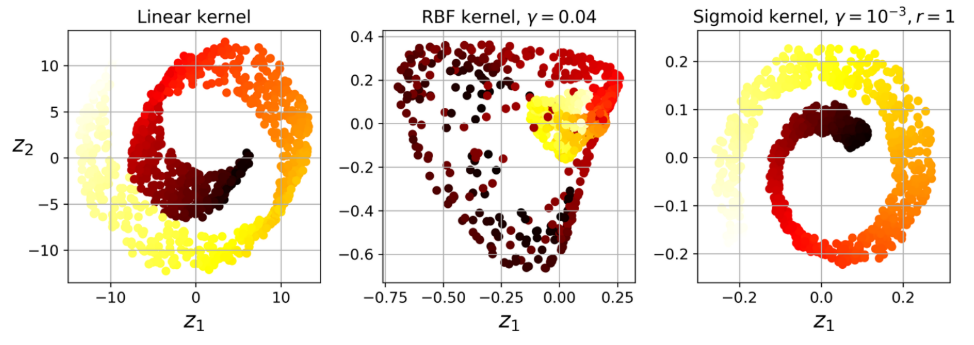
Kernel PCA

Kernel trick
- a mathematical technique that implicitly maps instances into a very high-dimensional space (called the feature space)
- a linear decision boundary in the high-dimensional feature space corresponds to a complex nonlinear decision boundary in the original space.
Benefits of kPCA
- It is often good at preserving clusters of instances after projection
- sometimes even unrolling datasets that lie close to a twisted manifold

Implementation

from sklearn.decomposition import KernelPCA 
rbf_pca = KernelPCA(n_components = 2, kernel="rbf", gamma=0.04)
X_reduced = rbf_pca.fit_transform(X)

example of different kernels

Other techniques

Locally Linear Embedding (LLE)

nonlinear dimensionality reduction (NLDR) technique
a Manifold Learning technique that does not rely on projections

Main idea

first measuring how each training instance linearly relates to its closest neighbors
then looking for a low-dimensional representation of the training set where these local relationships are best preserved.

Pros and Cons

Pro
- good at unrolling twisted manifolds, especially when there is not too much noise.
Con
- scale poorly to very large datasets

Implementation

from sklearn.manifold import LocallyLinearEmbedding 
lle = LocallyLinearEmbedding(n_components=2, n_neighbors=10) 
X_reduced = lle.fit_transform(X)

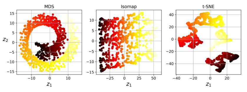
Other techniques

Random Projections
Multidimensional Scaling (MDS)
Isomap
t-Distributed Stochastic Neighbor Embedding (t-SNE)
Linear Discriminant Analysis (LDA)

Machine Learning: Dimensionality Reduction Techniques

Introduction to dimensionality reduction and python implementation

Importance

Main Approaches

PCA

PCA Idea

Randomized PCA

Incremental PCA

Kernel PCA

Other techniques

Locally Linear Embedding (LLE)

Other techniques

CATALOG

FEATURED TAGS

FRIENDS