Decision Trees can perform both classification and regression tasks, and even multioutput tasks.

Decision Trees don’t require feature scaling or centering.

Classification

Training and Visualization

from sklearn.datasets import load_iris
from sklearn.tree import DecisionTreeClassifier

iris = load_iris()
X = iris.data[:, 2:] # petal length and width
y = iris.target

tree_clf = DecisionTreeClassifier(max_depth=2, random_state=42)
tree_clf.fit(X, y)

# visualize
from graphviz import Source
from sklearn.tree import export_graphviz

export_graphviz(
        tree_clf,
        out_file=os.path.join(IMAGES_PATH, "iris_tree.dot"),
        feature_names=iris.feature_names[2:],
        class_names=iris.target_names,
        rounded=True,
        filled=True
    )

Source.from_file(os.path.join(IMAGES_PATH, "iris_tree.dot"))

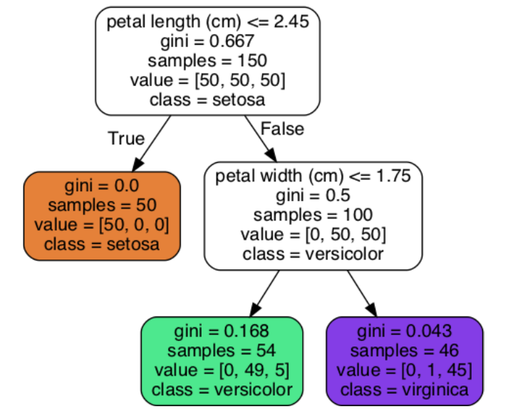
samples - how many training instances it applies to
value - how many training instances of each class this node applies to
class - prediction
gini - measures impurity

Gini impurity

This measures how pure your node is.
$G_i=1-\sum_k^np^2_{i,k}$ is gini $G_i$ of a node $i$, where $p^2_{i,k}$ is the ratio of class k instances among the training instances in the ith node.
A node is pure - gini=0 - if all training instances it applies to belong to the same class, for example, left node on depth 1.

Entropy

By default, the Gini impurity measure is used, but you can select the entropy impurity measure instead by setting the criterion hyperparameter to “entropy”
a set’s entropy is zero when it contains instances of only one class
Gini impurity is slightly faster to compute, so it is a good default
Gini impurity tends to isolate the most frequent class in its own branch of the tree, while entropy tends to produce slightly more balanced trees

Estimating class probabilities

First it traverses the tree to find the leaf node for this instance, and then it returns the ratio of training instances of class k in this node.

The CART Training algorithm

Scikit-Learn uses the Classification and Regression Tree (CART) algorithm to train Decision Trees (also called growing trees).

first splitting the training set into two subsets using a single feature $k$ and a threshold $t_k$
pair $(k, t_k)$ need to minimizes the cost function $J(k,t_k)=\frac{m_{left}}{m}G_{left}+\frac{m_{right}}{m}G_{right}$
Once the CART algorithm has successfully split the training set in two, it splits the subsets using the same logic, then the sub-subsets, and so on, recursively

Regularization

max_depth
min_samples_split - the minimum number of samples a node must have before it can be split
min_samples_leaf - the minimum number of samples a leaf node must have
min_weight_fraction_leaf - same as min_samples_leaf but expressed as a fraction of the total number of weighted instances
max_leaf_nodes - the maximum number of leaf nodes
max_features - the maximum number of features that are evaluated for splitting at each node

Notice Increasing min_* hyperparameters or reducing max_* hyperparameters will regularize the model

Regression

visualization

The main difference is that instead of predicting a class in each node, it predicts a value.

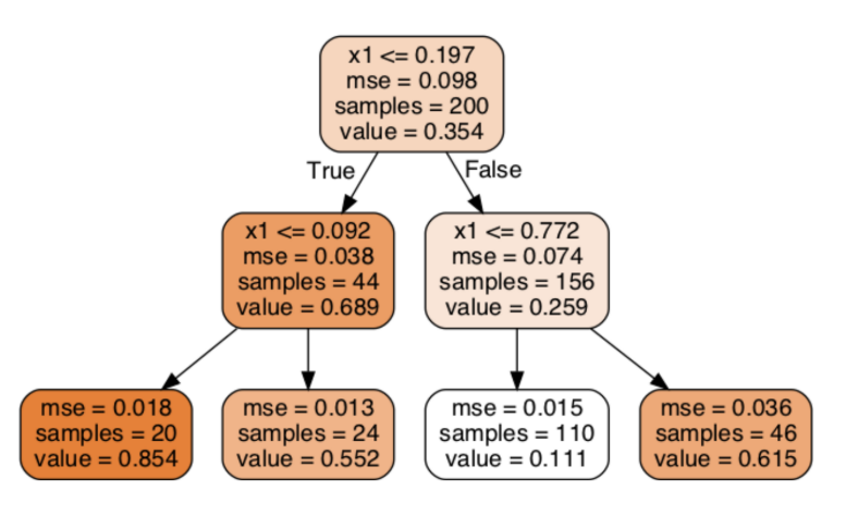
For example, suppose you want to make a prediction for a new instance with x1 = 0.6.

You traverse the tree starting at the root, and you eventually reach the leaf node that predicts value = 0.111.

This prediction is the average target value of the 110 training instances associated with this leaf node, and it results in a mean squared error equal to 0.015 over these 110 instances.

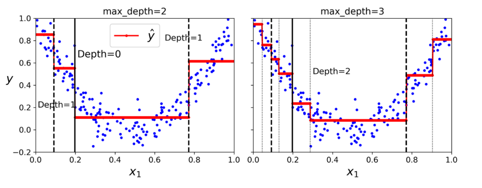
The fitted line is show below.

CART algorithm

The CART algorithm works mostly the same way as earlier, except that instead of trying to split the training set in a way that minimizes impurity, it now tries to split the training set in a way that minimizes the MSE.

\[J(k,t_k)=\frac{m_{left}}{m}MSE_{left}+\frac{m_{right}}{m}MSE_{right}\]

Some characteristics

Decision Trees don’t require feature scaling or centering.
easy to overfit
sensitive to training set rotation.
- because its decision boundaries are orthogonal (all splits are perpendicular to an axis
very sensitive to small variations in the training data
Random Forests can limit this instability by averaging predictions over many trees

Machine Learning: Decision Tree

A thorough introduction to Decision Tree

Classification

Regression

Some characteristics

CATALOG

FEATURED TAGS

FRIENDS