A Support Vector Machine (SVM) is a powerful ML model capable of performing linear or nonlinear classification, regression, and even outlier detection. It’s most significant characteristic is that SVMs are particularly well suited for classification of complex small or medium-sized datasets. Meanwhile, it does not scale well to big datasets.

Linear SVM Classification

The solid line in the plot on the right represents the decision boundary of an SVM classifier; this line not only separates the two classes but also stays as far away from the closest training instances as possible.

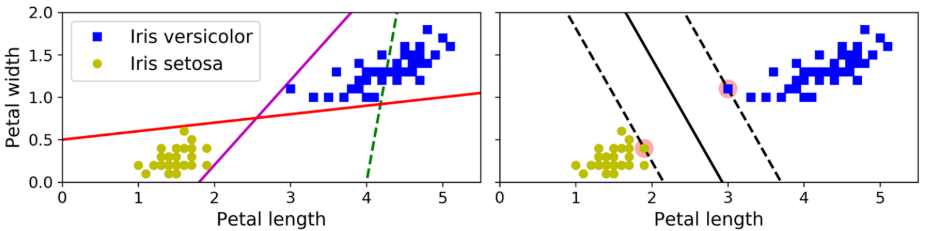
You can think of an SVM classifier as fitting the widest possible street (represented by the parallel dashed lines) between the classes. This is called large margin classification

Support vectors

• the instances located on the edge of the street
• these instances fully determine svm’s decision boundary
• adding more training instances “off the street” won’t affect decision boundaries

hard vs soft margin classification

• hard margin classification
  • strictly impose that all instances must be off the street and on the right side
  • two main issues
    • It only works if the data is linearly separable.
    • It is sensitive to outliers.
• soft margin classification
  • find a good balance between keeping the street as large as possible and limiting the margin violations
  • can be controlled by C parameter in sklearn SVM class
    • low C: wide street & many margin violations
    • high C: narrow street & fewer margin violations
  • Reducing C can help solving overfitting problem.

Python Code for Linear SVM

1
2
3
4
5
6
7
8
9
10
11
12
from sklearn.svm import LinearSVC, SVC
from sklearn.linear_model import SGDClassifier
# method 1
LinearSVC()

# method 2
SVC(kernel='linear', C=1, dual=False)
# Prefer dual=False when n_samples > n_features. 

# method 3
SGDClassifier(loss="hinge", alpha=1/(m*C))
# Defaults to ‘hinge’, which gives a linear SVM.

Notes

• SGDClassifier does not converge as fast as the LinearSVC class, but it can be useful to handle online classification tasks or huge datasets that do not fit in memory (out-of-core training)

Nonlinear SVM Classification

Many datasets are not linearly separable. We have two technique to solve nonlinear problems, corresponding to two kernel trick in SVM.

Polynomial kernel

Add more features, such as polynomial features to turn nonlinear datasets into linearly separable

implementation

1
SVC(kernel="poly", degree=3, coef0=1, C=5)

coef0: the importance of non-linear features compared to linear features

Gaussian RBF kernel

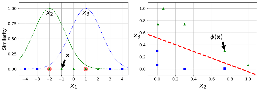
Similarity Features

Add features computed using a similarity function, which measures how much each instance resembles a particular landmark.

Similarity Function

Gaussian Radial Basis Function (RBF): $\phi_\gamma(x,l)=exp(-\gamma|x-l|^2)$ where $l$ is a landmark and we are measuring the similarity of the data point x with the landmark in the space of the original features.

This is a bell-shaped function varying from 0 (very far away from the landmark) to 1 (at the landmark).

Steps

• define similarity function
• choose landmarks, for example x1= –2 and x2 = 1
• for each point, calculate it’s new features according to landmarks. Instead of dealing with x as features of an instance, we shall use $\phi_γ(x, l_i)$ as features.
  • For example, there are two new features for point x=-1. One is its similarity with landmark 1 x1=-2, another is x1=1.
• Now we expand all 1d points into 2d plane (formed by similarity with two landmarks). And usually now the data will be linearly separable.

Downside

• A training set with m instances and n features gets transformed into a training set with m instances and m features (assuming you drop the original features).
• If your training set is very large, you end up with an equally large number of features.

Implementation

1
SVC(kernel='rbf', gamma=5, C=0.001)

• large gamma: narrow bell curve
• reduce gamma value can help solve overfitting as well, similar to C

SVM Regression

Instead of trying to fit the largest possible street between two classes while limiting margin violations, SVM Regression tries to fit as many instances as possible on the street while limiting margin violations (i.e., instances off the street)

• The width of the street is controlled by a hyperparameter $\epsilon$
  • large: wide street
• kernelized SVM can be used to tackle nonlinear regression tasks

Which kernel to select

• Try LinearSVC first. It is the fastest, especially if the training set is very large or if it has plenty of features
• If the training set is not too large, you should also try the Gaussian RBF kernel; it works well in most cases
• Other kernels exist but are used much more rarely
• Some kernels are specialized for specific data structures
• String kernels are sometimes used when classifying text documents or DNA sequences: the string subsequence kernel or kernels based on the Levenshtein distance.

A comparison of sklearn classes for svm

• Previous
  SQL For Interview (Strings)
• Next
  Machine Learning: Decision Tree