Linear Model

• Least squared method

  • define how to measure how well the model fits data. Let us use RMSE or MSE
  • find derivatives of MSE with respect to each parameter θ and set them to zero.
  • result in a system of linear equations

  • This closed-form solution is called a normal equation and can be written in a vector form as follows: $\hat{\theta}=(X^TX)^{-1}x^Ty$

  • Complexity: $O(n^{2.4})$ to $O(n^3)$, n is the number of features

• Singular Value Decomposition (used in sklearn)

  • uses matrix factorization to solve the system of equations to minimize MSE
  • complexity: $O(n^2)$

• Both methods scale linearly O(m) with the number of samples m.

• the predictions are very fast: linear in both n and m.

Gradient descent

• The general idea of Gradient Descent is to tweak parameters iteratively in order to minimize a cost function.
• gradient is a vector that points in the direction in which the error function would increase the most if we take a tiny step of size $η$
• learning rate: The size of the step we take $η$
  • When η is too small, it might take us a lot of steps to reach the minimum
  • When η is too large, it might keep overshooting the minimum
• Steps:
  • computes a gradient of the error function with respect to the parameters in the point of the parameter space
  • take a step in the direction opposite to where the gradient points: $\theta^{next step}= \theta - η\nabla_\theta Error(\theta)$
  • recompute gradient in the new point of the parameter space
  • keep iterating until we stop making progress in minimizing the error function
• Extra notes
  • Gradient descent can converge to a local optimum, even with a fixed learning rate. Because as we approach the local minimum, gradient descent will automatically take smaller steps as the value of slope i.e. derivative decreases around the local minimum.
  • The importance of feature scaling for GD to converge faster
  • MSE for linear regression is convex function, has no local minima but only one global minima. Therefore GD is guaranteed to converge to solution for sufficiently small learning rate if you wait long enough
• How to choose #of iterations
  • A simple solution is to set a very large number of iterations but to interrupt the algorithm when the gradient vector becomes tiny, smaller than some threshold $\epsilon$ called tolerance

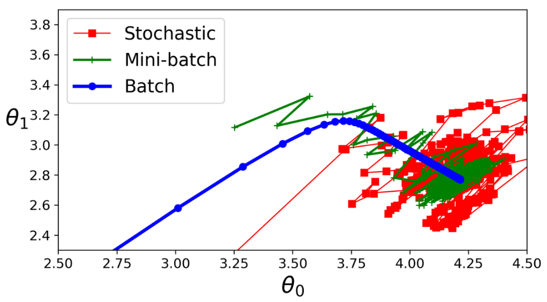
Stochastic Gradient Descent

• at each iteration it randomly selects one sample to compute error function on. Then as usual, take a step in the direction opposite to the gradient in the parameter space.
• Pros:
  • Can handle huge amount of data since it does not have to fit in memory
  • Good for online learning
  • Since it jumps all over the place, it has better chance of not been stuck in a local maxima
• Cons:
  • Since it jumps all over the place, it might never reach minimum
• Solution
  • One solution to insure that SGD converges is to start with the large learning rate but then keep reducing it.
  • The function that determines the learning rate at each iteration is called learning schedule.
  • If the learning rate is reduced too quickly, you may get stuck in a local minimum, or even end up frozen halfway to the minimum.
  • If the learning rate is reduced too slowly, you may jump around the minimum for a long time and end up with a suboptimal solution if you halt training too early.

Mini-batch Gradient Descent

• computes the gradients on small random sets of instances called mini-batches.
• Comparison with SGD
  • The main advantage of Mini-batch GD over Stochastic GD is that you can get a performance boost from hardware optimization of matrix operations, especially when using GPUs.
  • Mini-batch GD will end up walking around a bit closer to the minimum than Stochastic GD –
  • but it may be harder for it to escape from local minima

Regularization

Ridge Regression

• a regularized version of Linear Regression
• a regularization term equal to $\sum_{i=1}^n\theta^2_i $ is added to the loss function to penalize models with large θs.
• the regularization term should only be added to the error function during training
• \[Loss(\theta)=MSE(\theta)+\alpha \sum_{i=1}^n\theta^2_i\]
  • The hyperparameter α controls how much you want to regularize the model.
  • If α = 0, then Ridge Regression is just Linear Regression.
  • If α is very large, then all weights end up very close to zero and the result is a flat line going through the data’s mean.
  • The larger α is, the flatter and simpler the fit is

Lasso Regression

• another regularized version of Linear Regression
• it tends to eliminate the weights of the least important features
• \[Loss(\theta)=MSE(\theta)+\alpha \sum_{i=1}^n|\theta_i|\]

Elastic Net

• a middle ground between Ridge Regression and Lasso Regression
• \[Loss(\theta)=MSE(\theta)+r\alpha \sum_{i=1}^n|\theta_i| +\frac{1-r}{2}\alpha \sum_{i=1}^n\theta^2_i\]

1
2
3
4
5
6
7
8
9
# closed equation form in sklearn
RidgeRegression()
Lasso()
ElasticNet()

# sgd
SGDRegression(penalty="l2")
SGDRegression(penalty="l1")
SGDRegression(penalty="elasticnet")

How to choose among these regulariaztion?

• generally you should avoid plain Linear Regression.
• Ridge is a good default
• if you suspect that only a few features are useful, you should prefer Lasso or Elastic Net because they tend to reduce the useless features’ weights down to zero.
• Elastic Net is preferred over Lasso because Lasso might act erratically
  • when the number of features is greater than the number of training instances
  • when several features are strongly correlated.

Early stopping

• A very different way to regularize iterative learning algorithms such as Gradient Descent
  • stop training as soon as the validation error reaches a minimum - early stopping
• Another variation of this approach is to take checkpoints of the best model seen so far (in terms of the validation loss)

Logistic Regression

• Logistic Regression (also called Logit Regression) is commonly used to estimate the probability that an instance belongs to a particular class

• Just like a Linear Regression model, a Logistic Regression model computes a weighted sum of the input features (plus a bias term), but instead of outputting the result directly like the Linear Regression model does, it outputs the logistic of this result

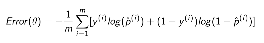
• For logistic regression, one typically uses log-loss error function instead of MSE

  

• no known closed-form equation to compute the value of θ that minimizes this cost function

• The error function is convex, so Gradient Descent (or any other optimization algorithm) is guaranteed to find the global minimum (if the learning rate is not too large and you wait long enough).

• LogisticRegression can be regularized with l1 or l2.

  • By default it is using l2
  • The parameter controlling the regularization is called “C” and it is inverse of α: the higher C, the less regularization

Softmax Regression

• support multiple classes directly, without having to train and combine multiple binary classifiers (generalization of logistic regression)

• Steps

  • Given an instance $X$, compute a score $s_k(X)$ for each class: $s_k(X)=X^T\theta ^{(k)}$

  • Note that each class has its own vector of parameters $θ^{(k)}$.

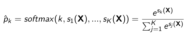
  • Then estimate the probability of each class by applying the softmax function - also called the normalized exponential - to the scores.

    

  • predicts the class with the highest estimated probability

• As an error function, cross-entropy is used

• Gradient Descent can be used to train Softmax Regression

1
LogisticRegression(multi_class="multinomial", solver="lbfgs", C=10)

• Previous
  Machine Learning: Classification Problem
• Next
  SQL For Interview (Strings)