Imbalanced dataset is a common problem in classification problem where there is a disproportionate ratio of samples in each class of y column. This could happen in cases like spam filtering, fraud detection.
In the case of class imbalance problems, the extensive issue is that the algorithm will be more biased towards predicting the majority class. The algorithm will not have enough data to learn the patterns present in the minority class.
In this blog, we will cover four possible ways to handle this problem in python specifically and discuss their use cases as well.
Change the performance metric
When we have imbalanced dataset, accuracy is not the best metric to use when evaluating imbalanced datasets as it can be very misleading. So Metrics that can provide better insight include:
- Confusion matrix
- a table showing correct predictions and types of incorrect predictions.
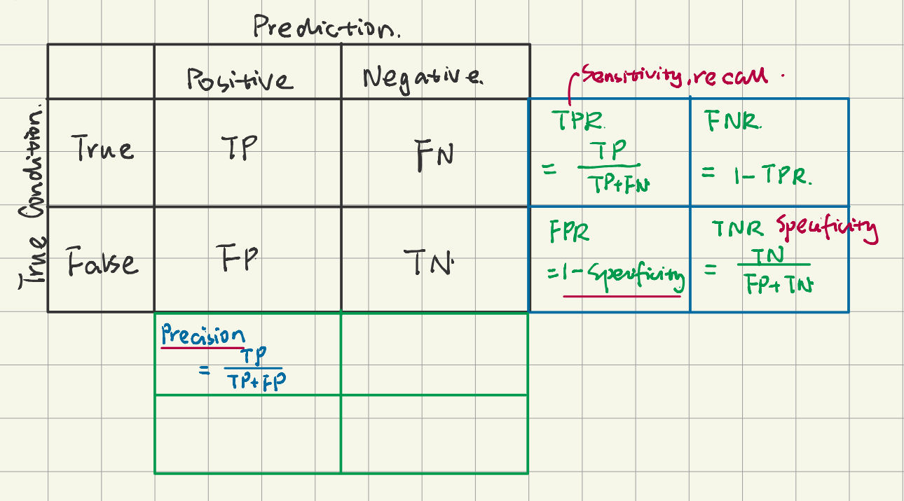
- Precision
- the number of true positives(TP) divided by all positive predictions
- a measure of a classifier’s exactness
- Low precision indicates a high number of false positives.
- Recall
- the number of true positives(TP) divided by the number of actually positive values
- also called Sensitivity or the True Positive Rate (TPR)
- a measure of a classifier’s completeness
- F1 score
- the weighted average of precision and recall.
- \[f1=\frac{precision\cdot recall}{precision+recall}\]
- PR AUC
- The area under PR curve
- PR (Precision-Recall) curve is a curve that combines precision (PPV) and Recall (TPR) in a single visualization. For every threshold, you calculate PPV and TPR and plot it. The higher on y-axis your curve is the better your model performance.
Among these four metrics, how should we choose the right metric for our problem? The general guidelines are:
- precision and recall can be chosen based on the specific business.
- high cost of false positive predictions: use precision
- high cost of false negative predictions: use recall
- f1 score can be chosen if there is no preference
- f1 score is more explainable than pr auc
Reference to this blog about the metrics comparison in classification problem.
Resampling Techniques
-
Random Over Sampling (ROS)
-
adding more copies of the minority class
-
1
2
3
from imblearn.over_sampling import RandomOverSampler
ros = RandomOverSampler(random_state=0, sampling_strategy='auto')
X_resampled, y_resampled = ros.fit_resample(X, y)
-
-
Random Under Sampling (RUS)
-
removing some observations of the majority class
-
1
2
3
from imblearn.under_sampling import RandomUnderSampler
rus = RandomUnderSampler(random_state=42)
X_res, y_res = rus.fit_resample(X, y)
-
Always split into test and train sets BEFORE trying oversampling techniques
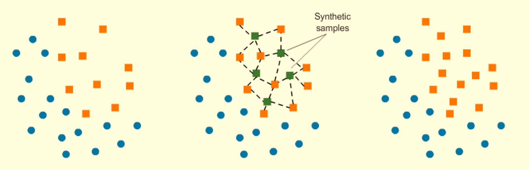
Generate synthetic samples (SMOTE)
-
Synthetic Minority Oversampling Technique
-
A technique similar to ROS
-
SMOTE uses a nearest neighbors algorithm to generate new and synthetic data we can use for training our model.
-
generate the new samples only in the training set
Comparison of ROS, RUS and SMOTE
-
Random Under Sampling (RUS): throw away data, computationally efficient
-
Random Over Sampling (ROS): straightforward and simple, but training your model on many duplicates
-
Synthetic Minority Oversampling Technique (SMOTE): more sophisticated and realistic dataset, but you are training on “fake” data (not on test set!)
Utilize sklearn parameters
- use parameter
class_weight - modify the current training algorithm to take into account the skewed distribution of the classes
- penalize the misclassification made by the minority class by setting a higher class weight and at the same time reducing weight for the majority class.
- values
class_weight=NoneBy defaultclass_weight=‘balanced’- \[w_j=n_{samples} / (n_{classes} * n_{samples_j})\]
- $w_j$ is the weight for each class(j signifies the class)
- $n_{samples}$ is the total number of samples or rows in the dataset
- $n_{classes}$ is the total number of unique classes in the target
- $n_{samples_j}$ is the total number of rows of the respective class
- pass a dictionary that contains manual weights for both the classes